This blog explains how to use the OpenAPI client in an SAP Data Intelligence data flow. Information about a specific location (point of interest), e.g. geo-coordinates, opening hours, websites are to be obtained with the help of GoogleMaps. It is thus shown how data can be enriched with additional information with the help of APIs.
This blog follows the following structure:
- Scenario in SAP Data Intelligence
- Prerequisites
- Structure
- Execution
- Outlook
Scenario in SAP Data Intelligence
SAP Data Intelligence (formerly Data Hub) is offered as a data management and pipeline solution. Data flows for orchestrating and monitoring data can be created flexibly and offer insights into the entire IT landscape through various connection options. In addition, these data flows can be cleansed, filtered, enriched, operationalized and optimized, leaving a solid database that can be leveraged by ML scenarios.
In Pipelines, there are many different operators that can perform the functions mentioned above. A large part of the operators is self-explanatory and easy to handle. However, there are other operators that are not so self-explanatory. One such case is the standard operator "OpenAPI Client". We will describe this in more detail with the GeoEnrichment use case.
For this blog, the Google Places API (Application Programming Interface) is to be used with the OpenAPI client. This can provide detailed information for a Place Id (Google internal unique ID).[1]
Requirements
In order to call a Google API, you first need a so-called API Key, with which you identify yourself for each call and are billed via the Google Account after a certain number of calls.[2],[3]
In addition, a Place ID must be available. This ID represents a specific location. This can be read with the Google Geocoding API from names and addresses or an example is taken from the documentation. In our case we take a Place ID from the official documentation.
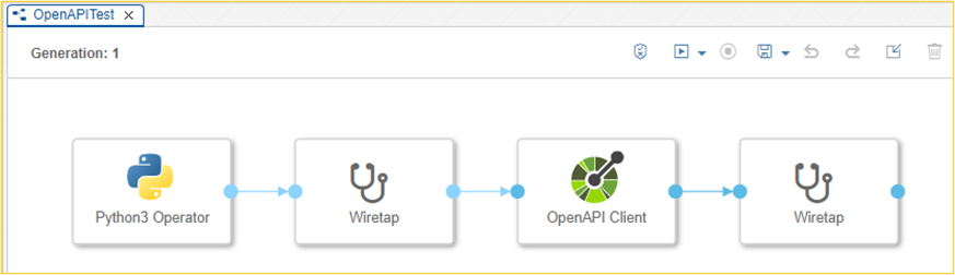
Structure of the graph
The structure of the graph takes place as follows:
- Python (Alternatively: JavaScript) operator to prepare the input parameters for the OpenAPI client operator.
- Optional wiretap to review the input parameters for the OpenAPI Client Operator
- OpenAPI Client Operator is the actual heart with the API call
- Optional wiretap to review the result of the API call
Calling the OpenAPI Client Operator
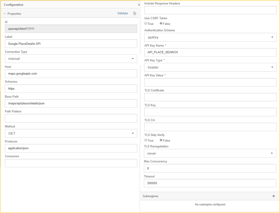
The first step is to configure the OpenAPI Client Operator. We select "manual" as the Connection Type to be able to maintain it directly. In productive operation, the connection parameters should be stored in the Connection Manager.[4] In the configuration area of the OpenAPI Client we have to fill Host, Schemes, Base Path, Method and Produces.
The filling of these fields can be understood with the documentation of the Google Place API already linked above. The figure below reflects an excerpt of the documentation, from which the areas of the URL with their corresponding meaning can be taken.
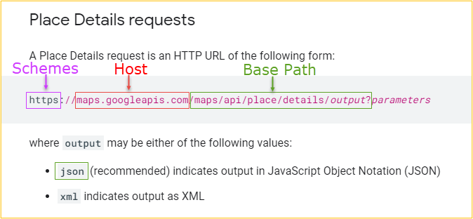
Abbildung 1: Eigene Darstellung in Anlehnung an Google Places Documentation
The "mandatory field" API Key Value is not filled directly in the OpenAPI client operator in this example. This is filled in the Python operator so that the input can also be scheduled as a parameter when starting the graph. The API Key Name can be freely chosen and "header" must be selected as API Key Type.
Python Operator
This now leads to the Python operator. This operator does not have to be configured or linked to a Dockerfile, but only adapted in the coding.
The OpenAPI client operator processes an input message. This is created in the code of the Python operator with the help of the "header" dictionary. The dictionary contains the API key and the place ID that are passed to the OpenAPI client.
The labels...
header[“openapi.query_params.key“] or
header[“openapi.query_params.place_id“]
follow a certain logic, which can be found in the OpenAPI Client Operator documentation.[5]
Additional header attributes can be used to pass more information for later processing. For example, we passed user and roles. The additional attributes have no influence on the result of the OpenAPI Client Operator and are therefore only passed on, but not processed.
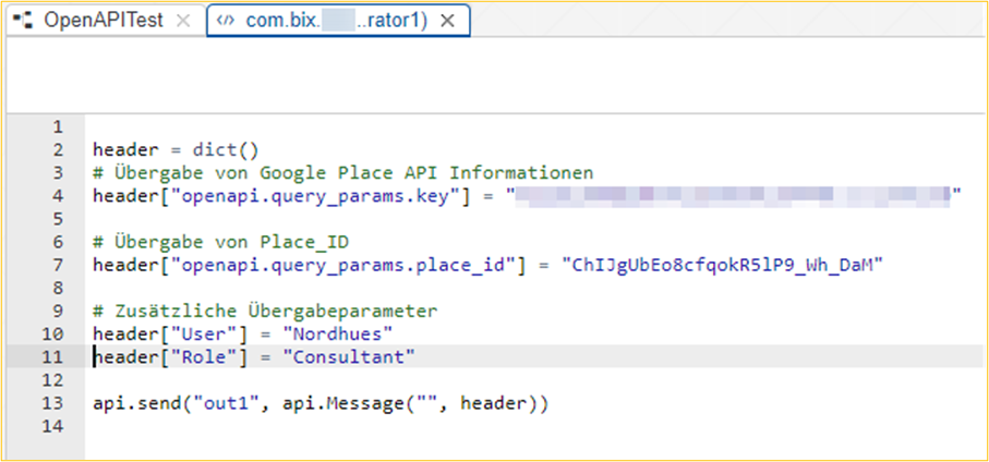
After realization of the configuration and implementation, the graph can be executed.
Execution
Once the graph has been executed, wiretaps can be used to view the various processing steps. The Python operator passes a message to the OpenAPI client operator, which was created from a dictionary in Python (see below). This message is the input to the OpenAPI Client Operator. The wiretap illustrates which information is passed and how. Also, it shows what can help with potential problems.
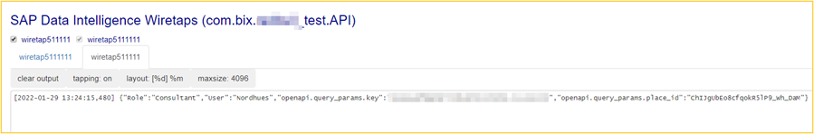
Result:
[2022-01-29 13:24:15,480]
{“Role“:“Consultant“, “User“:“Nordhues”, ”openapi.query_params.key”:”my_api_key”, ”openapi.query_params.place_id”:”ChIJgUbEo8cfqokR5lP9_wh_DaM”}
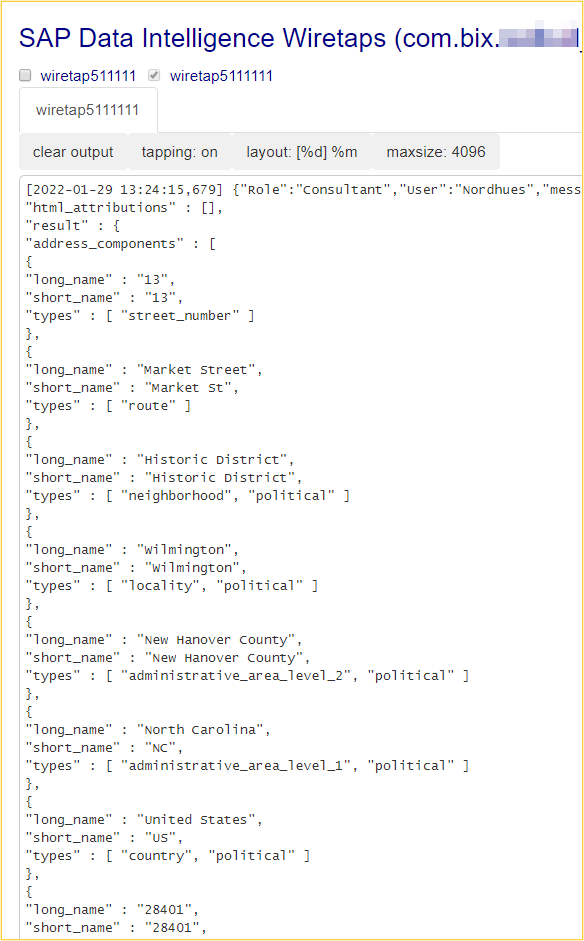
The OpenAPI client processes these results and outputs them in the final wiretap. The figure below shows only a small part of the delivered data.
Outlook
This example should be used as an example for further API's. The structure, after which API's are called, often does not differ. Accordingly, this example can also be used for other API's, for example What3Words.[6] It remains to be said that API guidelines are to be studied in detail, which defaults there are regarding storage and further processing of the API results.
Error handling
Further processing of the output string is more complex if we have a scenario where many API calls have to be made. Each OpenAPI client operator processes only single calls at a time, accordingly more operators need to be added in the graph. In addition, error handling functions must be implemented in case the OpenAPI client operator does not find a result.
Package processing
In a scenario where a simple graph is to process multiple records, it is necessary to wait until all records are processed before taking further steps. The Python operator initiates an API call for each record (through the OpenAPI Client operator). The step after the OpenAPI Client Operator is thus started for each row individually. Creativity is now required to ensure that all records have been processed and recollected before further steps follow.
Examples and scenarios
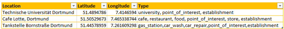
When using GeoEnrichment API's, you end up with a dataset that has been enriched with geo-data and other information about a specific location. This results in many different use cases. For example, the use of the map functionality in the SAC or distance calculations between different stores.
For example, in the figure below, longitude, latitude, and type of location were read for the three locations. This allows data sets to be built and filtered more granularly, so that sales can be reported by type, for example.
If you have any questions regarding the conception or implementation of SAP DI, please do not hesitate to contact us.
More information:
- Blog SAP Data Intelligence Cloud – OpenAPI Client Basics: https://blogs.sap.com/2021/09/13/sap-data-intelligence-cloud-openapi-client-basics/
- Documentation OpenAPI Client: https://help.sap.com/doc/de49c012b53d476eae7af14497eac256/2.4.latest/en-US/8a70738566e6466eb8d0f7d68be80247.html
Footnotes
1: https://developers.google.com/maps/documentation/places/web-service/details?hl=de (go to section)
2: Prices can only be found after logging into the Google Cloud Platform. They vary depending on the API and information requested. (go to section)
3: https://developers.google.com/maps (go to section)
4: https://help.sap.com/viewer/b13b5722c8ff4bf9bb097251310031d0/3.0.2/en-US/974be4fbb13a48eda16f7b061508eb59.html (go to section)
5: https://help.sap.com/viewer/97fce0b6d93e490fadec7e7021e9016e/Cloud/en-US/8a70738566e6466eb8d0f7d68be80247.html (go to section)
6: https://developer.what3words.com/public-api (go to section)
Contact Person


")


