In diesem Blog wird die Verwendung des OpenAPI Clients in einem SAP Data Intelligence Datenfluss erklärt. Es sollen mit Hilfe von GoogleMaps Informationen zu einem bestimmten Ort (Point of Interest), z.B. Geokoordinaten, Öffnungszeiten, Websiten eingeholt werden. Es wird somit gezeigt, wie mit Hilfe von API’s Daten um zusätzliche Informationen angereichert werden können.
Dieser Blog richtet sich nach folgender Struktur aus:
- Szenario in der SAP Data Intelligence
- Voraussetzungen
- Aufbau
- Ausführung
- Ausblick
Szenario in der SAP Data Intelligence
SAP Data Intelligence (ehemals Data Hub) wird als Datamanagement- und Pipelinelösung angeboten. Datenflüsse zur Orchestrierung und Überwachung von Daten lassen sich flexibel anlegen und bieten durch verschiedene Verbindungsmöglichkeiten Einblicke in die gesamte IT-Landschaft. Außerdem können diese Datenflüsse bereinigt, gefiltert, angereichert, operationalisiert und optimiert werden, sodass eine solide Datenbasis bleibt, welche von ML-Szenarien genutzt werden kann.
Im Bereich Pipelines gibt es viele verschiedene Operatoren, die die oben erwähnten Funktionen ausführen können. Ein großer Teil der Operatoren ist selbsterklärend und gut händelbar. Jedoch gibt es weitere Operatoren, die nicht so selbsterklärend sind. Ein solcher Fall ist der Standardoperator „OpenAPI Client“. Diesen wollen wir mit dem Anwendungsfall GeoEnrichment genauer beschreiben.
Für diesen Blog soll mit dem OpenAPI Client die Google Places API (Application Programming Interface) genutzt werden. Diese kann zu einer Place Id (Google interne eindeutige ID) detaillierte Informationen liefern.[1]
Vorraussetzungen
Um eine Google API aufzurufen, benötigt man als erstes einen sogennanten API Key, mit dem man sich für jeden Aufruf identifiziert und über den Google Account ab einer bestimmten Anzahl Aufrufe abrechnet.[2],[3]
Außerdem muss eine Place ID vorhanden sein. Diese repräsentiert als ID einen bestimmten Ort. Diese kann mit der Google Geocoding API aus Namen und Adressen gelesen werden oder es wird ein Beispiel aus der Dokumentation genommen. In unserem Fall nehmen wir eine Place ID aus der offiziellen Dokumentation.
Aufbau des Graphen
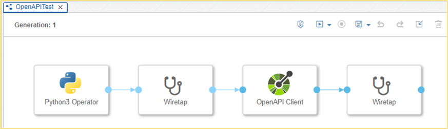
Der Aufbau des Graphen ist wie folgt:
- Python (Alternativ: JavaScript) Operator, um die Eingabeparameter für den OpenAPI Client Operator aufzubereiten
- Optionaler Wiretap erlaubt die Eingabeparameter für den OpenAPI Client Operator zu reviewen
- OpenAPI Client Operator ist das eigentliche Herzstück mit dem API-Aufruf
- Optionaler Wiretap um das Ergebnis, des API-Aufrufs zu überprüfen
Aufruf des OpenAPI Client Operator
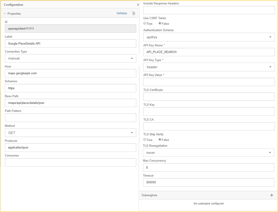
Als Erstes wird der OpenAPI Client Operator konfiguriert. Wir wählen als Connection Type „manual“ aus, um diese direkt pflegen zu können. Im produktiven Betrieb sollten die Verbindungsparameter im Connection Manager hinterlegt werden.[4] Im Konfigurationsbereich des OpenAPI Client müssen wir Host, Schemes, Base Path, Method und Produces befüllen.
Die Befüllung dieser Felder lässt sich mit der oben schon verlinkten Dokumentation der Google Place API nachvollziehen. Die untere Abbildung spiegelt ein Ausschnitt der Dokumentation wider, dem die Bereiche der URL mit ihrer entsprechenden Bedeutung entnommen werden können.
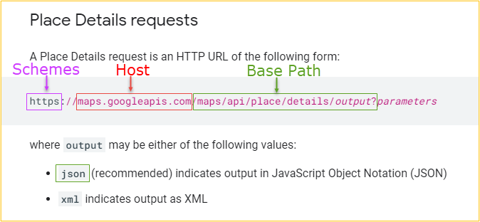
Abbildung 1: Eigene Darstellung in Anlehnung an Google Places Documentation
Das „Pflichtfeld“ API Key Value wird in dem OpenAPI Client Operator in diesem Beispiel nicht direkt gefüllt. Dies wird im Python Operator gefüllt, damit sich die Eingabe auch als Parameter beim Start des Graphen planen lässt. Der API Key Name kann frei gewählt werden und es muss „header“ als API Key Type gewählt werden.
Python Operator
Dies führt nun zum Python Operator. Dieser muss nicht extra konfiguriert oder mit einem Dockerfile verknüpft, sondern lediglich im Coding angepasst werden.
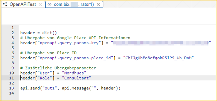
Der OpenAPI Client Operator verarbeitet eine Input Message. Diese wird im Code des Python Operators mit Hilfe des Dictionary „header“ erstellt. Das Dictionary enthält den API-Key und die Place ID die den OpenAPI Client übergeben werden.
Die Bezeichnungen…
header[“openapi.query_params.key“] oder
header[“openapi.query_params.place_id“]
folgen einer bestimmten Logik, die man der Dokumentation zum OpenAPI Client Operator entnehmen kann.[5]
Durch zusätzliche Headerattribute können weitere Informationen zur späteren Verarbeitung weitergegeben werden. Beispielsweise haben wir User und Rollen übergeben. Die zusätzlichen Attribute haben keinen Einfluss auf das Ergebnis des OpenAPI Client Operator und werden somit nur weitergegeben, aber nicht prozessiert.
Nach Umsetzung der Konfiguration und Implementierung kann der Graph ausgeführt werden.
Ausführung
Wenn der Graph ausgeführt wurde, kann man sich mit Hilfe der Wiretaps die verschiedenen Verarbeitungsschritte ansehen. Der Python Operator übergibt dem OpenAPI Client Operator eine Message, die aus einem Dictionary in Python erstellt wurde (siehe unten). Diese Message ist der Input für den OpenAPI Client Operator. In dem Wiretap ist veranschaulicht, welche Informationen wie übergeben werden und was bei möglichen Problemen helfen kann.
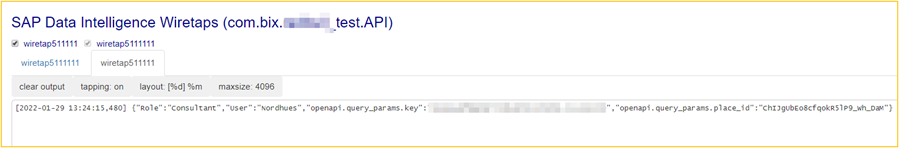
Ergebnis:
[2022-01-29 13:24:15,480]
{“Role“:“Consultant“, “User“:“Nordhues”, ”openapi.query_params.key”:”my_api_key”, ”openapi.query_params.place_id”:”ChIJgUbEo8cfqokR5lP9_wh_DaM”}
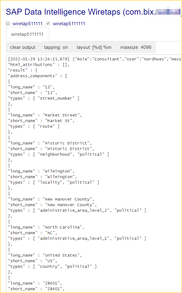
Der OpenAPI Client verarbeitet diese Ergebnisse und gibt diese im letzten Wiretap aus. Die untere Abbildung zeigt nur einen kleinen Ausschnitt der gelieferten Daten.
Aussicht
Dieses Beispiel soll exemplarisch für weitere API’s genutzt werden. Die Struktur, nach denen API’s aufgerufen werden, unterscheidet sich oftmals nicht. Dementsprechend kann dieses Beispiel auch für weitere API’s, beispielweise What3Words, verwendet werden.[6] Festzuhalten bleibt es, dass API-Richtlinien genaustens zu studieren sind, welche Vorgaben es bzgl. Speichern und Weiterverarbeitung der API-Ergebnisse gibt.
Fehlerbehandlung
Die weitere Verarbeitung des Ausgabestrings ist aufwendiger, wenn wir ein Szenario haben, indem viele API-Aufrufe gemacht werden müssen. Jeder OpenAPI Client Operator verarbeitet immer nur einzelne Aufrufe, dementsprechend müssen weitere Operatoren in dem Graph hinzugefügt werden. Zusätzlich müssen Errorhandling-Funktionen umgesetzt werden, falls die OpenAPI Client Operator kein Ergebnis findet.
Paketverarbeitung
In einem Szenario, in dem ein einfacher Graph mehrere Datensätze verarbeiten soll, muss gewartet werden, bis alle Datensätze verarbeitet sind, bevor weitere Schritte unternommen werden. Der Python Operator stößt für jeden einzelnen Satz einen API-Aufruf an (durch den OpenAPI Client Operator). Der Schritt nach dem OpenAPI Client Operator wird dadurch für jede Zeile einzeln gestartet. Jetzt ist Kreativität gefragt, um sicherzustellen, dass alle Datensätze verarbeitet und wieder gesammelt wurden, bevor weitere Schritte folgen.
Beispiele und Szenarien
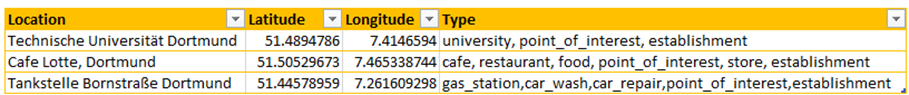
Bei der Verwendung von GeoEnrichment API‘s, hat man am Ende ein Datenset, welches mit Geo-Daten und weiteren Informationen zu einem bestimmten Ort angereichert wurde. Daraus ergeben sich viele verschiedene Anwendungsbeispiele. Zum Beispiel die Nutzung der Karten-Funktionalität in der SAC oder Distanzberechnungen zwischen verschiedenen Stores.
In der unteren Abbildung wurden zum Beispiel für die drei Orte Längen- und Breitengrade sowie der Typ des Ortes ausgelesen. Dadurch wird ermöglicht, Datensätze granularer aufzubauen und zu filtern, sodass beispielsweise Umsätze nach Typen reportet werden können.
Falls Sie Fragen zur Konzeption oder Umsetzung rund um das Thema SAP DI haben, sprechen Sie uns gerne an.
Weitere Informationen:
- Blog SAP Data Intelligence Cloud – OpenAPI Client Basics: https://blogs.sap.com/2021/09/13/sap-data-intelligence-cloud-openapi-client-basics/
- Dokumentation OpenAPI Client: https://help.sap.com/doc/de49c012b53d476eae7af14497eac256/2.4.latest/en-US/8a70738566e6466eb8d0f7d68be80247.html
Fußnoten
1: https://developers.google.com/maps/documentation/places/web-service/details?hl=de (zum Abschnitt)
2: Preise lassen sich erst nach Anmeldung auf der Google Cloud Plattform finden. Sie variieren je nach API und abgefragten Informationen. (zum Abschnitt)
3: https://developers.google.com/maps (zum Abschnitt)
4: https://help.sap.com/viewer/b13b5722c8ff4bf9bb097251310031d0/3.0.2/en-US/974be4fbb13a48eda16f7b061508eb59.html (zum Abschnitt)
5: https://help.sap.com/viewer/97fce0b6d93e490fadec7e7021e9016e/Cloud/en-US/8a70738566e6466eb8d0f7d68be80247.html (zum Abschnitt)
6: https://developer.what3words.com/public-api (zum Abschnitt)
Ansprechpartner


")


