Introduction
Machine learning is an important part of exhausting the full value of big data. Advanced algorithms can be used to gather all kinds of information from almost any kind of data source. However, the process of gathering the data, making the data usable and training models on the data is not so easily done. Hence a sophisticated machine learning life cycle is already an achievement, but a platform which can be used for all steps of the life cycle is even rarer. Though, Databricks provides in this aspect.
Databricks is a cloud development environment for data engineers, data scientists and data analysts. It can be deployed on multiple cloud environments like Azure or AWS. Databricks mainly uses Spark functionalities for engineering, python and MLFlow for machine learning and SQL queries for analysis. One of many benefits of Databricks is that different teams like data engineers and data scientists can collaborate in one environment to be able to produce an entire machine learning life cycle together. However, since the compute capacities in Databricks are provided by clusters, which take a certain time to start, deploying machine learning models can be very costly and time inefficient. This is not really a problem when models are served for batch inference, however when models are to be served on demand, efficiency is key and there is a solution for that.
In this blog an experiment will be described in which a machine learning project was prepared and executed in Databricks and deployed using azureml. The case used for the experiment is to predict which team wins in a team-based video game. In this video game two teams of five players compete against each other to take out hostile objectives and slay the enemy characters with the ultimate goal to destroy the enemies’ base. While each team progresses, the individual players also progress their characters to become stronger. The experiment tries to predict which team wins based on the data of the first ten minutes of a game. Here the main characteristics of a winning or losing team are the strength of the players’ individual characters and the progression of their team.
This case may seem unusual for the topics biX normally covers, however when test cases are created for research purposes, the topics can be chosen freely. So, in this case a certain video game was chosen for the experiment for reasons of general interest, accessibility of the data and complexity of the case.
Data Extraction and Preparation
The data used for this experiment is extracted from an API. This extraction is coded in a Databricks notebook using the requests library of python. After the immediate extraction, the data is partly turned directly into a Spark dataframe, the rest of the data must first be flattened using the function pandas.json_normalize and other means of extracting columns and rows in an orderly manner into dataframes, since most of the data is structured in the JSON format. After converting all of the data into Spark dataframes they can be persisted in the Azure blob storage as Delta Tables (df.write.format(‘delta’).write()). Delta Tables have the benefit of acting like tables in a relational database (including data warehouse functions like change data capturing (cdc)) even when saved in a blob storage.
Of course, before any of the aggregations are performed, the data is thoroughly analysed: What are the ranges of each column? What types do the columns have? How do the columns correlate with each other? Which columns are useful and which are obsolete? All these question can be answered by importing the data into a Databricks notebook and performing investigative data analysis with either Spark, SQL or python. For this the display() function can also be utilized to visualize the results of the explorations.
In machine learning you can rarely ever use the data sets as they are. Most of the time data needs to be analysed, aggregated, and prepared. In this case most of the actions are: Taking averages and totals over columns as well as adding weights to certain rows to accentuate their impact on the machine learning model. To be concrete with an example: The stats of the characters in earlier stages of the game are less important than the stats later on, which is why the more recent stats are weighted more. These aggregations are done by using the Spark Dataframe API.
Finally, the data needs to be saved as a delta table to be easily accessible. However, the transformed data will be made even easier to use with the Feature Store in Databricks. Here data can either be saved as or get linked to a feature store, where data can flexibly be pulled out to create training sets for machine learning that are replicable. The feature store is especially useful in the context of performing multiple experiments since the same training data can be used an unlimited amount of time without having to re-code time consuming data extractions and transformations. By being able to add tags, mark data set keys and have access to the notebook which created a feature store data set (even with versioning) a lot of time is saved and functionality won.
Machine Learning
To begin with the machine learning, the transformed input data will be loaded into a new notebook. By using the feature store for this, the experiments in this notebook will be easily replicable. Therefore, an instance of the feature_store is created. After that mlflow autolog will be enabled to record parameters and metrics of experiments in this notebook. Now the mlflow run will be started, meaning that all of the following code will be replicable in the Experiments section.
Within the run the training set is loaded from the feature store, the data set is divided into training and test data, the parameters are set, the model is trained, and the performance is evaluated: The training set is loaded by using a self-defined lookup and a set of ids as reference (create_training_set()). Then the sklearn function train_test_split is used to split the data into a training and a test data set. After that the parameters for the experiment are set. These will be changed around a lot to make sure that the resulting model is as optimal as possible. Luckily the parameters are also tracked in MLflow Experiments, so that when the best model is chosen, all details are available and the model can be loaded at any other point of time in other any other notebook or scenario with minimal coding. Going on, the model needs to be initialized and trained. In this case multiple experiments with different models will be created, to ensure a good prediction quality. Decision trees, random forests and support vector machines are being tested. Finally, at the end of each experiment the newly created model is used to predict results for the test data set. By doing this the difference between the predictions and the actual correct values can be calculated to create metrics that specify the precision of the model. Multiple metrics are calculated (accuracy, precision, recall, f-measure) and then logged using mlflow.log_metrics().
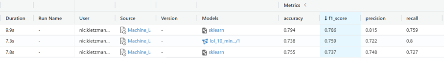
The Screenshot shows the metrics for experiments with Random Forest, Decision Tress and Support Vector Machines in the mentioned order.
Even though many different experiments were executed, it is easily possible to choose the best models from them. For each used type of algorithm (decision tree, random forest, support vector machine), one model is chosen simply by looking at the recorded metrics. The random forest has the best results in the end, however the decision tree can be used to explain which features are impacting the decision making due to the ability to visualize it. Visualizations show that teams which earn a lot of gold in a match, have a higher chance to win. The same goes for the inflicted physical damage. This may sound very straight forward but in a game with 1000s of different variables it is not easy to assume how even the simplest factors influence the outcome of a match. The impact of the described features can be seen in the following:
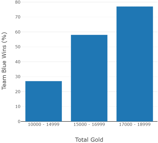
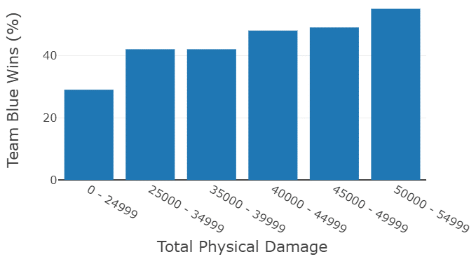
The probabilities to win rise clearly with the rise of the given features. Like already discussed, this video game has countless variables in every match, so seeing such a clear result is very surprising.
Deployment
To make the newly trained model accessible it now needs to be deployed. Of course, one possibility for this would be to deploy the model on a cluster in Databricks, however two problems arise with that solution: Letting Databricks clusters run 24/7 is extremely expensive, which rules this variant out, additionally having to start a Databricks cluster every time shortly before you want to use it is also inefficient due to the clusters taking three to five minutes to start.
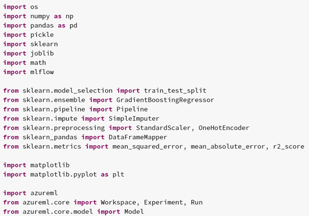
To avoid the problems of deploying the model on Databricks, the model is instead deployed on azureml. azureml will permanently run the service to grant instant access to the model and generate way less costs at the same time. The code for preparing the service is written and executed in Databricks. Firstly, azureml and all necessary underlying functions are imported:
Then the Workspace is defined in which the model and webservice will be deployed. The definition contains information like which Azure subscription will be used:
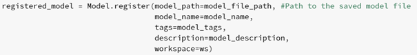
After that, the already trained model can be registered to azureml by providing the path, name, and other information:
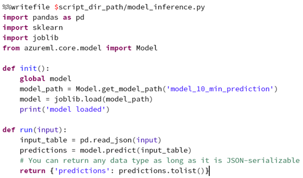
Now a very interesting part follows: Code-snippets (initial and run) need to be provided to the webservice, so that the code for running the service initially and the code for answering requests is set. The code snippets can contain operations on the input data, the actual inference on the input data, or data transformations for the output, basically anything can be inserted here, making the service extremely flexible:
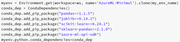
Remaining are the prerequisites for starting the webservice. The Environment (which packages and functions are used):
The configuration of the inference (containing the Environment information and the path to the initial and run code):
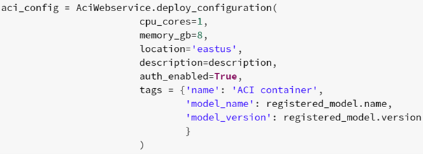
The configuration of the Webservice (number of cores, RAM, model):
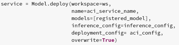
The Webservice (name, model, configuration) itself:
Finally, when everything is done and the service is running, an API-key can be generated, which will be used to access the service and for example send fresh match data from our video game to receive the prediction of which team will win.
All in all Databricks provides a lot of comfortable benefits for Machine Learning. With the Feature Store and mlflow experiments can be versioned and replicated in a manageable fashion. The deployment can be done in Databricks as well, using azureml. The flexible code snippets for this part creates countless possibilities. Additionally teams can work very close together since data scientists, data analysts and data engineers can all work in one platform.
Now neither the victory of our favourite team nor the efficiency of our machine learning services are up to chance.
If you have any question concerning machine learning or Databricks features like the feature store, please feel free to contact us.
Contact Person


")


