
Creation and use of autoencoders with SAP PAL

Data sets to be used in Machine Learning (ML) are usually unprocessed and immensely large in practice. Most ML algorithms require the input data in a specific form, which is provided by data preprocessing. Even then, however, the data model at hand is usually very complex.

Another problem with data sets can be the lack of balance between classes. In a classification project, the respective ML algorithm is fed a data set that has a class attribute in addition to regular attributes and an index. For example, in a customer churn analysis. Here, all tuples are provided with a value, whether the respective customer has churned or not, the class attribute. However, if the data set for the customer churn analysis is not balanced and, for example, only 20% of the customers churn, this can lead to inaccuracies in the resulting model with the ML algorithm used. In order to simultaneously counteract the problems of the high complexity of data sets and the lack of balance, autoencoders can be created with the help of the SAP Predictive Analysis Library (PAL).

An autoencoder is an artificial neural network (KNN). As shown in Figure 1, an autoencoder consists of five elementary components. The original data, the encoder, the reduced data, the decoder and the reverse engineered original data. Unlike traditional KNNs, the target is not the last layer of the network, but the middle layer. When training the autoencoder, the original data is used both as input to the first layer and as the target for the last layer. In the remaining layers, the data is reduced, compressed and then mapped back as best as possible. In the middle layer of the KNN, there is thus a reduced form of the original data with fewer dimensions. Autoencoders are usually used for anomaly analysis and noise reduction (filtering of noise values/elements). (https://towardsdatascience.com/auto-encoder-what-is-it-and-what-is-it-used-for-part-1-3e5c6f017726)
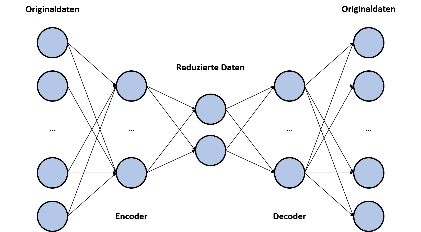
 

Figure 1: Components of an autoencoder

In the scenario we worked on, a data set was used for customer churn analysis. Together with the index and the class attribute, the dataset has 21 attributes, such as gender, length of customer relationship, monthly cost, etc. Before the dataset was processed by SAP PAL, the attribute characteristics were scaled. Thus, all attributes were scaled between 0.3 and 0.7, except for the class attribute, which was scaled between 0 and 1 to focus on this attribute. A KNN was then created using SAP PAL based on the dataset. To create such a network, only the input data, a parameter table and an empty table for the resulting model are necessary. The KNN is then stored by SAP PAL in json format in the model table, divided into several rows of 5000 characters each. The model table was then exported and disassembled using simple means in Python to be imported back into the HANA database as separate model tables for the encoder and decoder. However, this step can also be performed as needed using SQL without exporting in the system itself. By using the PREDICT procedure of SAP PAL, the two models could be used. In this way, the 19-dimensional data model (21 minus index and class attribute) could be converted to a two-dimensional data set using the encoder.

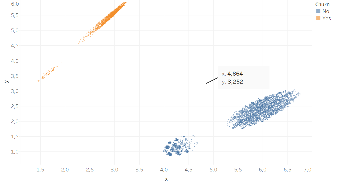
Figure 2 shows the data set used in coded form. In addition, a utility of the autoencoder is also shown. A random tuple was selected from the dataset and a feature expression was set to 13 (which is well above the scaled maximum 0.7), clearly representing an outlier, an anomaly. Using the PREDICT procedure, the two-dimensional expressions for this tuple could be calculated. It clearly stands out among the rest of the data points.

Another benefit of the autoencoder is also evident in Figure 2. Adding more tuples to the data set used is not a problem in the two-dimensional representation. If tuples of the class of churning customers are needed, they can simply be added to the corresponding cluster. This is particularly easy in this case because a focus was placed on the class attribute during the previous scaling and the tuples were thus automatically sorted strongly according to this by the KNN. If new tuples have been added as desired, the tuples can be translated back into the original dimensions with the decoder.
Churn, Tupel

Figure 2: Representation of the coded data set

Conclusion

Autoencoders can be used for various purposes and are easy to create with SAP PAL. Splitting the model created by SAP PAL into encoders and decoders can be costly depending on the implementation, but can be handled as a one-time effort using appropriate SQL procedures. In the case of anomaly analysis, it is particularly important to emphasise how visually the analysis can be operated, since a two-dimensional representation of coded data is easy to implement. In the scenario we practically implemented, the data set used could be supplemented in two-dimensional form with tuples of a certain class (bouncing customers). After conversion with the decoder, the extended data set had then produced significantly improved results in the ML algorithm used for customer churn analysis. The added tuples, moreover, strongly resembled the existing tuples, which meant that the data set was not too heavily distorted by generated tuples.

Contact Person

Oliver Ossenbrink

Management of sales and HR

Data Products Setup

I’ll start with Data Products setup. If you’re new to the concept, this recent video is a great starting point, but here’s a short summary. A data product is a well-described, easily discoverable, and consumable collection of data sets.

Creating a Data Product in Datasphere

Note that in this article I create Data Products in the Data Sharing Cockpit in Datasphere. This functionality is expected to move into the Data Product Studio, but that had not taken place at the time writing.

Before creating a Data Product in Datasphere, I need to set up a Data Provider profile, collecting descriptive metadata like contact and address details, industry, regional coverage, and importantly define Data Product Visibility. Enabling Formations allows me to share the Data Product with systems across your BDC Formation – Databricks, in this case.

With the Data Provider set up, I can go ahead and create a Data Product. As with the Data Provider, I’ll need to add metadata about the product and define its artifacts – the datasets it contains. Only datasets from a space of SAP HANA Data Lake Files type can be selected. Since this Data Product is visible across the Formation, it is available free of charge.

For this demo, the artifact is a local table containing ten years of Ice Cream sales data. Since this is a File type space, importing a CSV file directly to create a local table isn’t an option (see documentation).

I used a Replication Flow to perform an initial load from a BW aDSO table into a local table.

Once Data Product is created and listed, it becomes available in the Catalog & Marketplace, from where it can be shared with Databricks by selecting the appropriate connection details.

Jump into Databricks

To use the shared object In Databricks, I need to mount it to the Catalog – either by creating a new Catalog or using an existing one.

Databricks appends a version number to the end of the schema – ‘:v1’ – to maintain versioning in case of any future changes to the Data Product.

Once the share is mounted, the schema is created automatically, and the Sales actual data table becomes available within it. From there, I can access the shared table directly in a Notebook.

Creating a Data Product in Databricks

To create a Data Product in Databricks, I first need to create a Share – which I can either do via the Delta Sharing settings in the Catalog:

Or directly out of the table which is going to become a part of the Share:

Since a single Share can contain multiple tables, I have the option to either add the table to an existing Share, or create a new one:

To publish the Share as a Data Product, I run a Python script where I define the target table for the forecast and describe the Share in CSN notation, setting the Primary Keys. Primary Keys are required for installing Data Products in Datasphere.

Jump back into Datasphere

Once the Databricks Data Product is available in Datasphere, I install it into a Space configured as a HANA Database space – since my intention is to build a view on top of the table and use it for planning in SAC.

There are two installation options: as a Remote table for live data access, or as a Replication Flow, in which case the data is physically copied into the object store in Datasphere.

Since I want live access, I install it as a Remote Table:

and build a Graphical view of type Fact on top:

Forecast calculation

With my Data Products set up and Sales actual data are available in Databricks, I create a Notebook to calculate the Sales Forecast.

The approach combines Sales and Weather data to train a Linear Regression model. I import the Weather data *https://zenodo.org/records/4770937 from an external server directly into Databricks, select the relevant features from the weather dataset, and combine them with the Sales actual data:

* Klein Tank, A.M.G. and Coauthors, 2002. Daily dataset of 20th-century surface
air temperature and precipitation series for the European Climate Assessment.
Int. J. of Climatol., 22, 1441-1453.
Data and metadata available at http://www.ecad.eu

Using the “sklearn” library, I build and train a Linear regression model:

Once trained, the model predicts the Sales forecast for Rome in June 2026 based on the weather forecast, and I save the results to my Catalog table:

Seamless planning data model

Seamless planning concept is built around physically storing planning data and public dimensions directly in Datasphere, keeping them alongside the actual data.

Since the QRC4 2025 SAC release, it has also been possible to use live versions and bring reference data into planning models without replication.

In this scenario, I build a seamless planning model on top of the Graphical view I created over the Remote table. This lets me use the forecast generated in Databricks as a reference for the final SAC Forecast version.


The model setup follows these steps:

Create a new model:

Start with data:

Select Datasphere as the data storage:

From there, I define the model structure and can review the data in the preview.

For a deeper dive into Seamless Planning, I recommend this biX blog.

Process Flow automation

Multi-action triggers Datasphere task chain

The final step is automating the entire forecast generation by using SAC Multi-actions and a Task-Chain in Datasphere – so that my user can trigger the calculation with a single button click from an SAC Story.

The model setup follows these steps:

Create a new model:

Triggering Task Chains from Multi-actions is a recent release. This blog post walks through how to set it up.

For details on how to trigger a Databricks Notebook from Datasphere, I recommend referring to this blog.

With everything in place, I create a Story, add my Seamless planning Model, and attach the Multi-action:

Running the Multi-action triggers the Task Chain, which in turn triggers the Databricks Notebook.

I can monitor the execution details in Datasphere:

and in Databricks:

Once the calculation completes, the updated forecast appears in the Story:

The end-to-end calculation took 2 minutes 45 seconds in total. The Task Chain in Datasphere is triggered almost instantly by the Multi-action, the Databricks Notebook execution itself took 1 minute 29 seconds, with the remaining time spent on Serverless Cluster startup.   


From here, I can copy the calculated forecast into a new private version:

adjust the numbers as needed, and publish it as a new public version to Datasphere:

Conclusion

With SAP Business Data Cloud, it is possible to build a forecasting workflow that feels seamless to the end user — even though it spans multiple systems under the hood.

Companies using BW as the main Data Warehouse and Databricks for ML calculations or Data Science tasks can benefit from using the platform, as the data no longer needs to be physically copied out of BW.

What this scenario demonstrates is that once wrapped as a Data Product, BW sales data can be shared with Databricks via the Delta Share protocol. Databricks, in turn, can then create its own Data Products on top of the calculation results and share them back with Datasphere as a Remote Table.

A Seamless Planning model in SAC sits on top of that Remote Table, giving planners live access to the generated forecast. A single Multi-action in an SAC Story ties it all together, triggering a Datasphere Task Chain that kicks off the Databricks Notebook — completing the full cycle in under three minutes.

As SAP Business Data Cloud continues to mature, scenarios like this one are becoming achievable – leaving the complexity in the architecture and not in the workflow.

Contact

Ilya Kirzner
Consultant
biX Consulting
Privacy overview

This website uses cookies so that we can provide you with the best possible user experience. Cookie information is stored in your browser and performs functions such as recognizing you when you return to our website and helps our team to understand which sections of the website are most interesting and useful to you.