Let’s install an Open Source infrastructure for the SAP Datahub on-premise – Part 2 of 2

This is the second part of our article in which we explain, how to install an SAP Datahub on an Open Source infrastructure. The following expects that you successfully have a Kubernetes cluster running and additionally, fulfil all other requirements for the installation. Not sure? you are welcome to start with part 1: Basic thoughts, installation steps and checkpoints for the Datahub infrastructure.

Installing and configuring the so called in the installation guide “Jump Host”:

This is a Linux machine with the requirement of at least 50GB for the images (registry). However, to be on the safer side use a bigger disk. Here is the filesystem usage after all steps are completed (to get the estimation for the size):

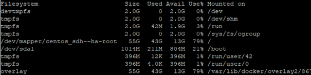
For this machine I have used CentOS 7, updated to the latest version. As every SAP system that uses SAP Host Agent, it is needed to have the correct record in the DNS and hosts file. After this we will be able to start the setup. Few abbreviations will be used in this document: DH – Data Hub, HA – Host Agent, JH – jump host, Kubernetes Cluster – KC, SAP Maintenance Planner – MP.

JH is going to be used for few things:

Transfer and execute the MP’s generated XML
Installation host – where the setup is executed, and commands are sent to the KC
Registry (as repository), where the Docker images will be downloaded from SAP and stored to be provided to the KC
Registry for the used apps by DH

Same as any other SAP system installation, we start by logging in MP. We select Plan a new system -> Plan:

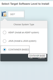
Here the container-based option is selected, after this the SID is automatically set to CNT. Then we must select the product – SAP DATA HUB is the only option. After this – the version – 2:

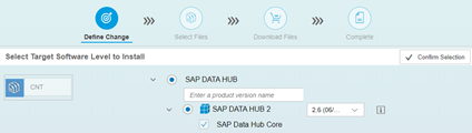
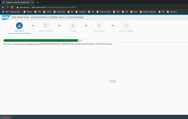
After confirming the action, we continue with the standard procedure of pushing the files to the download basket followed by the step of ‘Execute Action’ selection. After clicking on it, we will have to get the address and port settings to be filled – in our case the hostname of the JH and the port of the Host Agent. At this very moment, when selecting Deploy of the XML file from the MP, the feature called CORS (Cross Origin Resource Sharing) will be used. After successful result, when reloading the web of the JH, we will get the following option:

As you can see, the XML from the MP is transferred, and the selected version is displayed with its patch level.

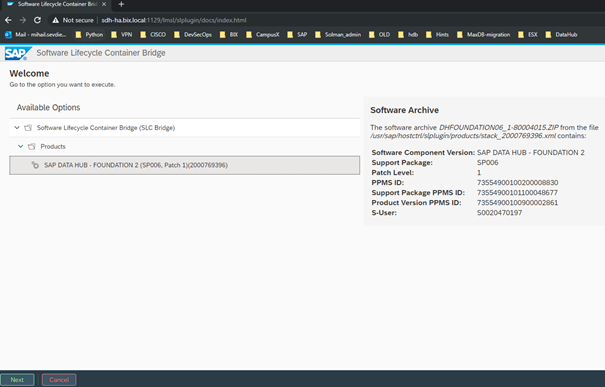
We can now start the process of installation using the Next Button.

The first step is to provide the S-User and this will be needed to download the files from SAP’s Launchpad needed for the installation media for DH and later – for the Docker image repository, to download the images to our local Docker registry.

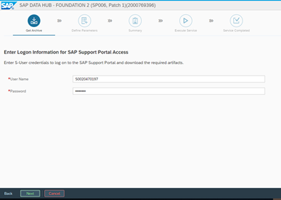
The process is pretty quick, since it now only downloads the needed ZIP archive. Alternatively, this can be done manually and the files can be uploaded in the SLC bridge folder. However, we have internet access, therefore we will use the option of automatic download.

Successful download is confirmed by the version info of the file:

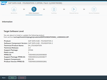
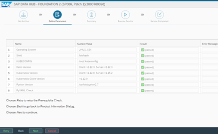
We confirm by clicking ‘Next’ and find ourselves in the step of the verification. By using the KC config file, the prerequisites are checked and if there are problems with the version compatibility there will be a warning. In our case it is all good, so we can continue.

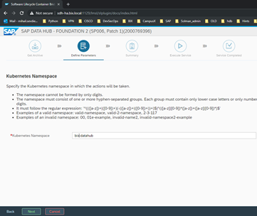
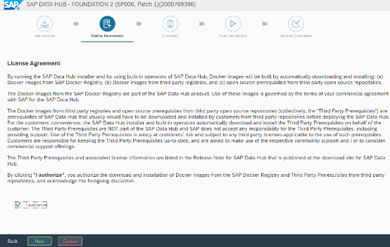
The next step is to select the name of the KC namespace, that will be used for the DH and after this we have the License Agreement to check:

After selecting I authorize, we can proceed to the next step:

We can select Advanced installation and after this we have to select “Do Not use” on the next step for the repository images. This will set the option to download the images. If we use offline installation, we have to select to use the already downloaded images. On the next steps, we have to provide again the S-User that is going to be used for downloading the images for Docker.

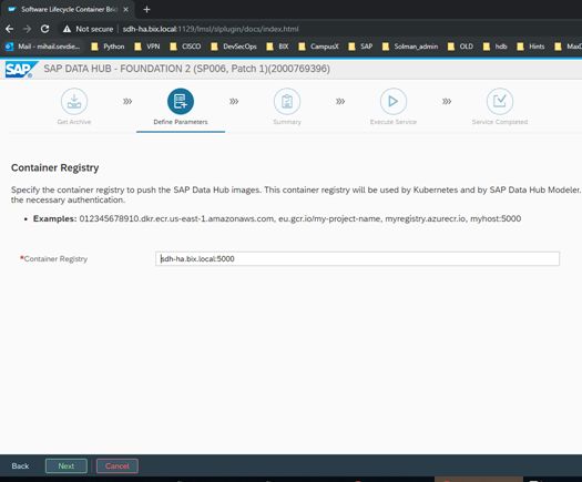
After this we have to provide the local Registry’s address.

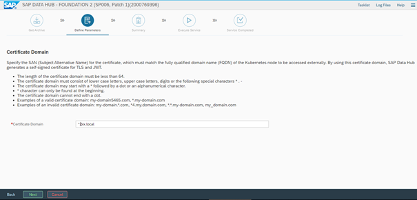
Next we have to choose the certificate domain for the installation.

On the next steps contain the required tenant name and admin details for it. Two tenants will be created – one system and one user’s tenant. The system one can be used for creating more client’s tenants. In our case we will create a tenant with the name “bix-consulting” and we will set username for administration to be admin with a strong password.

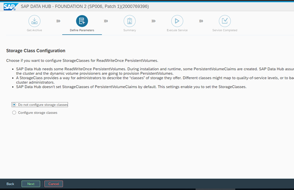
The next prompts are for Cluster proxy settings – we are not going to use ones, so we can select “Do not configure” and also, we will not use checkpoint storage configuration.

After this, we will be prompted for the Storage Class used for the installation. In our case we have configured the KC to have a default one, so we will let the setup to detect the default one and use it for the persistent volumes:

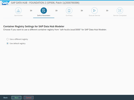
On the next step, we can set the Docker registry used for the Data Hub Modeler. It can be different from the one used for the installation, but in our case, we will use the same one:

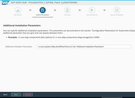
Then we select to Load the NFS modules (default selection) and set custom parameters. They are available in the SAP’s DH installation guide. In our case we will use only one parameter:

After this we can review our input and start the process if we don’t have to make any changes. It will begin with copying the Docker images into the local Repository (catalog):

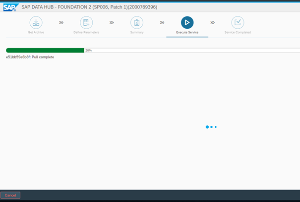
And then it will start to deploy the images on the KC:

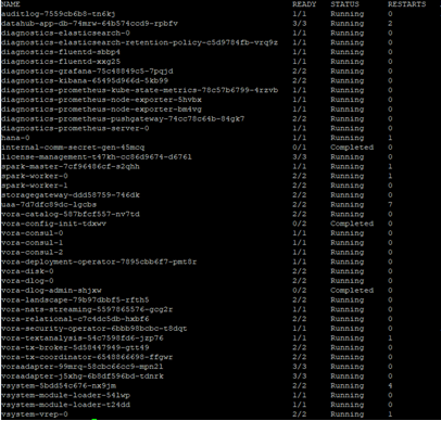
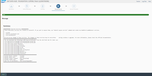
If everything is running fine, the setup will have the following result:

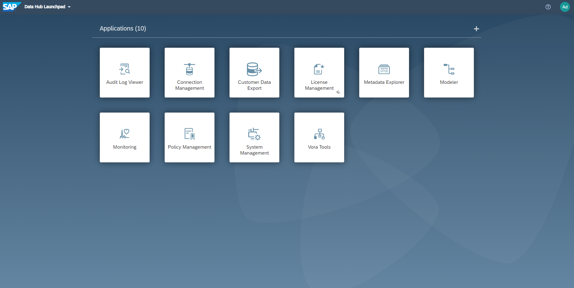
After this, we have to expose the web service to the nodes and login into the system:

We can test the installation by starting a demo application for generating random numbers. It should bring up a pod and start the code there. It is important to note, that after completing a task, we should stop it and then delete the pod from the web interface, otherwise the pod will stay in the KC with status Completed.

By completing the Modeler test, the SAP Datahub installation is finished successfully. We would appreciate any kind of comments and hope, you enjoyed reading. See you soon!

Ansprechpartner

Oliver Ossenbrink

Geschäftsführung Vertrieb und HR

Data Products Setup

I’ll start with Data Products setup. If you’re new to the concept, this recent video is a great starting point, but here’s a short summary. A data product is a well-described, easily discoverable, and consumable collection of data sets.

Creating a Data Product in Datasphere

Note that in this article I create Data Products in the Data Sharing Cockpit in Datasphere. This functionality is expected to move into the Data Product Studio, but that had not taken place at the time writing.

Before creating a Data Product in Datasphere, I need to set up a Data Provider profile, collecting descriptive metadata like contact and address details, industry, regional coverage, and importantly define Data Product Visibility. Enabling Formations allows me to share the Data Product with systems across your BDC Formation – Databricks, in this case.

With the Data Provider set up, I can go ahead and create a Data Product. As with the Data Provider, I’ll need to add metadata about the product and define its artifacts – the datasets it contains. Only datasets from a space of SAP HANA Data Lake Files type can be selected. Since this Data Product is visible across the Formation, it is available free of charge.

For this demo, the artifact is a local table containing ten years of Ice Cream sales data. Since this is a File type space, importing a CSV file directly to create a local table isn’t an option (see documentation).

I used a Replication Flow to perform an initial load from a BW aDSO table into a local table.

Once Data Product is created and listed, it becomes available in the Catalog & Marketplace, from where it can be shared with Databricks by selecting the appropriate connection details.

Jump into Databricks

To use the shared object In Databricks, I need to mount it to the Catalog – either by creating a new Catalog or using an existing one.

Databricks appends a version number to the end of the schema – ‘:v1’ – to maintain versioning in case of any future changes to the Data Product.

Once the share is mounted, the schema is created automatically, and the Sales actual data table becomes available within it. From there, I can access the shared table directly in a Notebook.

Creating a Data Product in Databricks

To create a Data Product in Databricks, I first need to create a Share – which I can either do via the Delta Sharing settings in the Catalog:

Or directly out of the table which is going to become a part of the Share:

Since a single Share can contain multiple tables, I have the option to either add the table to an existing Share, or create a new one:

To publish the Share as a Data Product, I run a Python script where I define the target table for the forecast and describe the Share in CSN notation, setting the Primary Keys. Primary Keys are required for installing Data Products in Datasphere.

Jump back into Datasphere

Once the Databricks Data Product is available in Datasphere, I install it into a Space configured as a HANA Database space – since my intention is to build a view on top of the table and use it for planning in SAC.

There are two installation options: as a Remote table for live data access, or as a Replication Flow, in which case the data is physically copied into the object store in Datasphere.

Since I want live access, I install it as a Remote Table:

and build a Graphical view of type Fact on top:

Forecast calculation

With my Data Products set up and Sales actual data are available in Databricks, I create a Notebook to calculate the Sales Forecast.

The approach combines Sales and Weather data to train a Linear Regression model. I import the Weather data *https://zenodo.org/records/4770937 from an external server directly into Databricks, select the relevant features from the weather dataset, and combine them with the Sales actual data:

* Klein Tank, A.M.G. and Coauthors, 2002. Daily dataset of 20th-century surface
air temperature and precipitation series for the European Climate Assessment.
Int. J. of Climatol., 22, 1441-1453.
Data and metadata available at http://www.ecad.eu

Using the “sklearn” library, I build and train a Linear regression model:

Once trained, the model predicts the Sales forecast for Rome in June 2026 based on the weather forecast, and I save the results to my Catalog table:

Seamless planning data model

Seamless planning concept is built around physically storing planning data and public dimensions directly in Datasphere, keeping them alongside the actual data.

Since the QRC4 2025 SAC release, it has also been possible to use live versions and bring reference data into planning models without replication.

In this scenario, I build a seamless planning model on top of the Graphical view I created over the Remote table. This lets me use the forecast generated in Databricks as a reference for the final SAC Forecast version.

The model setup follows these steps:

Create a new model:

Start with data:

Select Datasphere as the data storage:

From there, I define the model structure and can review the data in the preview.

For a deeper dive into Seamless Planning, I recommend this biX blog.

Process Flow automation

Multi-action triggers Datasphere task chain

The final step is automating the entire forecast generation by using SAC Multi-actions and a Task-Chain in Datasphere – so that my user can trigger the calculation with a single button click from an SAC Story.

The model setup follows these steps:

Create a new model:

Triggering Task Chains from Multi-actions is a recent release. This blog post walks through how to set it up.

For details on how to trigger a Databricks Notebook from Datasphere, I recommend referring to this blog.

With everything in place, I create a Story, add my Seamless planning Model, and attach the Multi-action:

Running the Multi-action triggers the Task Chain, which in turn triggers the Databricks Notebook.

I can monitor the execution details in Datasphere:

and in Databricks:

Once the calculation completes, the updated forecast appears in the Story:

The end-to-end calculation took 2 minutes 45 seconds in total. The Task Chain in Datasphere is triggered almost instantly by the Multi-action, the Databricks Notebook execution itself took 1 minute 29 seconds, with the remaining time spent on Serverless Cluster startup.

From here, I can copy the calculated forecast into a new private version:

adjust the numbers as needed, and publish it as a new public version to Datasphere:

Conclusion

With SAP Business Data Cloud, it is possible to build a forecasting workflow that feels seamless to the end user — even though it spans multiple systems under the hood.

Companies using BW as the main Data Warehouse and Databricks for ML calculations or Data Science tasks can benefit from using the platform, as the data no longer needs to be physically copied out of BW.

What this scenario demonstrates is that once wrapped as a Data Product, BW sales data can be shared with Databricks via the Delta Share protocol. Databricks, in turn, can then create its own Data Products on top of the calculation results and share them back with Datasphere as a Remote Table.

A Seamless Planning model in SAC sits on top of that Remote Table, giving planners live access to the generated forecast. A single Multi-action in an SAC Story ties it all together, triggering a Datasphere Task Chain that kicks off the Databricks Notebook — completing the full cycle in under three minutes.

As SAP Business Data Cloud continues to mature, scenarios like this one are becoming achievable – leaving the complexity in the architecture and not in the workflow.