SQL im Composite Provider – Mächtige Funktion aber evtl. überraschende Berechnungen

In einem Composite-Provider kann man nun neue Merkmale oder Kennzahlen per eigenem SQL füllen! 

Dies ist eine spannende Funktion, mit der man viele Anforderungen elegant lösen kann. Verwendet man dies bei Kennzahlen, kann es jedoch passieren, dass das Ergebnis nicht ganz den Erwartungen entspricht und sich sogar noch verändert, wenn man andere Kennzahlen mit in den Aufriss nimmt. Daher soll hier mit einem einfachen Beispiel das Verhalten analysiert und erklärt werden. Dann steht eine Verwendung dieser mächtigen Funktion ohne „böse“ Überraschung auch nichts mehr im Weg.  

Der Blog ist wie folgt aufgebaut:

  • Vorstellung der neuen Funktionalität
  • Erklärung des kleinen Beispiels
  • Überraschende Ergebnisse
  • Vermeidung der falschen“ Berechnung

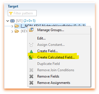
Die neue Funktionalität

Wenn das BW/4 auf ausreichendem Patch-Level ist (HANA 2.0 SPS 04), sieht man folgende neue Option im Composite Provider: 

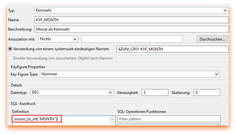
Um aus einem nummerischen Attribut eine Kennzahl zu erzeugen, reicht nun folgendes SQL: 


snumc_to_int( „ATTRIBUTE_NUMC“ ) 


Damit ist der Composite-Provider noch einmal viel mächtiger geworden und vermeidet wohl häufig die Verwendung eines Calculation Views oder erspart das Anlegen und Füllen einer neuen Kennzahl / eines neuen Merkmals im aDSO. Insbesondere die Vermeidung des Calculation Views hilft, nicht noch eine weitere Technik einzuführen. Außerdem ist nicht immer der Zugriff direkt auf die HANA gewünscht.  

Diese Funktion findet man in den SAP–Release Informationen (https://help.sap.com/viewer/b3701cd3826440618ef938d74dc93c51/2.0.6/de-DE/d8b12ec099e04e6aa77a312be687db63.html) und in diesem schönen Blog https://www.brandeis.de/en/blog/sql-expressions-in-bw-4hana-composite-provider-hcpr/  gut beschrieben. 

Kleines Beispiel

Schauen wir uns das Verhalten an folgendem Beispiel einmal an. (Das Beispiel erhebt keinen Anspruch auf fachlichen Sinn, es sollen nur mit einfachen Zahlen und Rechnungen die Ergebnisse leicht nachvollziehbar sein ?. Ebenso gibt es evtl. für die Fragestellungen noch andere Lösungsansätze, aber diese sollen hier nicht betrachtet werden. Wir möchten nur die Funktion der SQL–Verarbeitung nachvollziehen!). 

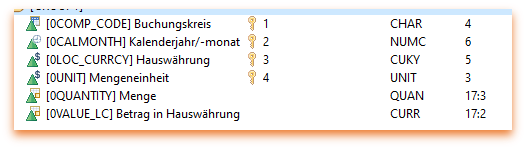
Wir haben ein aDSO, das wie folgt aufgebaut ist: 

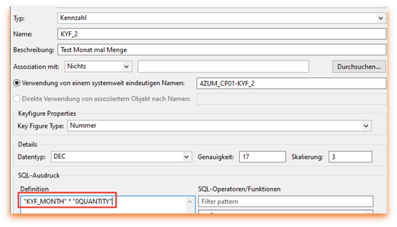
Nun wollen wir folgende Kennzahlen im Calculation View ergänzen: 

Menge mit dem Monat gewichten, d.h. Menge im Januar * 1, Februar *2 etc. 

Damit alle Schritte kontrolliert werden können, sind diese als einzelne Merkmale bzw. Kennzahlen angelegt. Dies wäre natürlich auch in einem Schritt möglich 

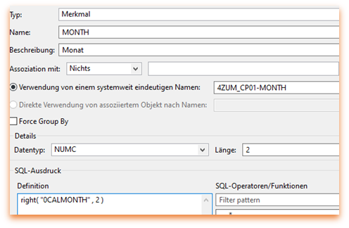
In einem ersten Schritt holen wir aus 0CALMONTH den Monat. 

Danach wandeln wir den Monat in eine Kennzahl um.

Zum Abschluss noch mit der Menge multiplizieren.

In einem weiteren Beispiel sollen die Einträge mit EUR als Währung gezählt werden, d.h. die Kennzahl soll immer 1 enthalten, wenn die Währung EUR enthält. Dies ist mit folgender SQL–Anweisung möglich: 


CASE „0LOC_CURRCY“ 

          WHEN ‚EUR‘ THEN 1 

          ELSE 0 

 END 

Überraschende Ergebnisse

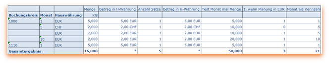
Sind alle Attributte aufgerissen, dann erfolgt die Berechnung, wie wir sie intuitiv erwarten:

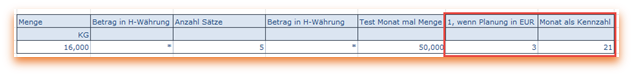
Werden keine Attribute in der einfachen Query / Listcube angezeigt, bekommt man folgendes Ergebnis: 

  • die Zählung der Monate mit EUR liefert einen Monat zu wenig (vorletzte, erwartet 4, nun 3)
  • die Summe der Monate als Kennzahl kommt zu einem anderen Ergebnis (letzte Spalte, erwartet 22, nun 21)

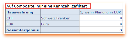
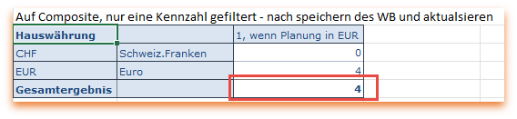
Noch verwirrender wird es, wenn man sich nur die Kennzahl zur Zählung der Monate mit EUR anschaut und die Währung anzeigt.  Beides mal haben wir in den Zeilen die Währung, in der Spalte nur die eine Kennzahl, aber Achtung:  

  • Der Bericht auf dem Composite, der die Kennzahl filtert, liefert das erwartete Ergebnis von 4, in der Summe, allerdings nur 3!
  • Speicher man das Workbook und frischt es wieder auf, so wird das Gesamtergebnis auf einmal wie erwartet mit 4 angezeigt
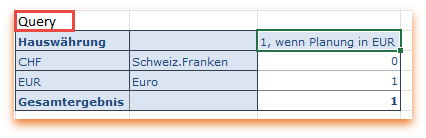
  • Eine Query mit nur einer Kennzahl in den Spalten liefert aber nur 1.

Ursache für die  „falschen“ Ergebnisse

Um die Performance zu optimieren, werden die Daten immer zuerst so weit wie möglich aggregiert und dann wird das SQL für die neuen Merkmale im Composite-Provider ausgeführt.

Werden also zwei Attribute in der Berechnung benötigt, dann werden die Daten auf diese Ebene aggregiert, die Berechnung durchgeführt und dann weiter aggregiert, wenn dies für die Anzeige nötig ist. 

Die Berechnung aller verwendeten Kennzahlen wird auf derselben Ebene ausgeführt, d.h. wenn mehrere Berechnungen durchgeführt werden müssen, dann wird nur so weit aggregiert, dass alles gleichzeitig berechnet werden kann. 

Dies führt dazu, dass die Berechnungen unterschiedlich ausfallen können, ja nachdem, welche Kennzahlen gleichzeitig angezeigt werden sollen. Sind alle Merkmale im Aufriss, dann erfolgt die Berechnung auf der untersten Ebene. 


In unserem Fall werden der Monat und die Währung benötigt, um die Berechnung für alle Formeln wie erwartet durchzuführen. Wenn daher alle Kennzahlen vorkommen, aber keine Merkmale im Aufriss sind, wird zuerst auf diese Ebene verdichtet. Dass wir im Januar in zwei Buchungskreisen Zahlen in EUR haben, ist egal, da diese Zeile nur einmal vorkommt und damit nur einmal gezählt wird. Daher erhalten wir hier nur einen 3 statt der 4. Lässt man noch die Währung anzeigen, dann scheint noch eine weitere Logik bei den Einzelzeilen zu ziehen, die hier nun wieder zu einer 4 führt. Noch verwirrender wird es, wenn man diese Darstellung abspeichert und wieder aktualisiert. Dann ist auf einmal auch das Gesamtergebnis richtig. 

Haben wir nur die Kennzahl zur Zählung der EUR–Zahlen in der Query angefordert, dann erfolgt hier eine Verdichtung bis auf die Währung, bevor das SQL ausgeführt wird. Daher erhalten wir die 1 für einmal Ausprägung EUR.

„Richtige“ Berechnung erzwingen

Zum Glück gibt es die Möglichkeit, die Query zu überzeugen, „korrekt“ zu rechnen. 

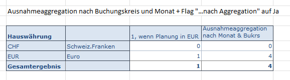
Hierfür müssen zwei Einstellungen geändert werden. Zuerst legen wir eine Formel an, die die eigentliche Kennzahl übernimmt und für die wir die Ausnahmeaggregation definieren: 

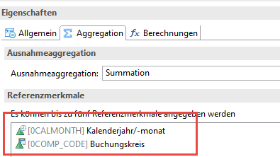
Als Referenzmerkmale sind alle Merkmale anzugeben, die wir bei der Berechnung berücksichtigen möchten. Da hier maximal 5 Merkmale erlaubt sind, ist dieses Vorgehen sicher nicht für jedes Modell geeignet. Aber häufig benötigen wir hier nicht alle Merkmale des Modells, sondern nur diejenigen, die sich unabhängig unterscheiden können, bzw. die bei der Zählung zu berücksichtigen sind. So reicht z.B. in vielen Modellen vermutlich die Belegnummer. 

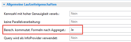
Allein mit dieser Ausnahmeaggregation erfolgt erstaunlicherweise immer noch keine korrekte Berechnung. Erst, wenn im Reiter Laufzeiteigenschaften der Query die Einstellung „Berech. Kommutat. Formel nach Aggregat.:“ auf Ja gestellt wird, kommt das „richtige“ Ergebnis heraus: 

Ob man die Berechnung auf unterer Ebene erzwingen kann, indem man die Merkmale in der Formel anspricht oder diese einer Kennzahlen zuordnet, für die eine Ausnahmeaggregation hinterlegt ist, haben wir nicht versucht. Wie immer gibt es sicher noch viele weitere Möglichkeiten an das Ziel zu kommen. 

Unabhängig von der hier vorgestellten Lösung, kann solch eine Fragestellung häufig auch in einer Query mit Formeln gelöst werden. Dies ist aber dann auf eine einzelne Query beschränkt und mit ähnlichen Einschränkungen behaftet. 


Fazit 

Auch wenn die Erklärungen und das Verhalten zuerst verwirrend klingt,  folgt die Software wie immer einfachen Regeln ?. Hat man diese Verstanden, dann kann die neue Funktionalität ohne „böse“ Überraschung verwendet werden. Viel Spaß dabei! 

Ansprechpartner

  Dr. Ulrich Meseth

   Senior Consultant

Data Products Setup

I’ll start with Data Products setup. If you’re new to the concept, this recent video is a great starting point, but here’s a short summary. A data product is a well-described, easily discoverable, and consumable collection of data sets.

Creating a Data Product in Datasphere

Note that in this article I create Data Products in the Data Sharing Cockpit in Datasphere. This functionality is expected to move into the Data Product Studio, but that had not taken place at the time writing.

Before creating a Data Product in Datasphere, I need to set up a Data Provider profile, collecting descriptive metadata like contact and address details, industry, regional coverage, and importantly define Data Product Visibility. Enabling Formations allows me to share the Data Product with systems across your BDC Formation – Databricks, in this case.

With the Data Provider set up, I can go ahead and create a Data Product. As with the Data Provider, I’ll need to add metadata about the product and define its artifacts – the datasets it contains. Only datasets from a space of SAP HANA Data Lake Files type can be selected. Since this Data Product is visible across the Formation, it is available free of charge.

For this demo, the artifact is a local table containing ten years of Ice Cream sales data. Since this is a File type space, importing a CSV file directly to create a local table isn’t an option (see documentation).

I used a Replication Flow to perform an initial load from a BW aDSO table into a local table.

Once Data Product is created and listed, it becomes available in the Catalog & Marketplace, from where it can be shared with Databricks by selecting the appropriate connection details.

Jump into Databricks

To use the shared object In Databricks, I need to mount it to the Catalog – either by creating a new Catalog or using an existing one.

Databricks appends a version number to the end of the schema – ‘:v1’ – to maintain versioning in case of any future changes to the Data Product.

Once the share is mounted, the schema is created automatically, and the Sales actual data table becomes available within it. From there, I can access the shared table directly in a Notebook.

Creating a Data Product in Databricks

To create a Data Product in Databricks, I first need to create a Share – which I can either do via the Delta Sharing settings in the Catalog:

Or directly out of the table which is going to become a part of the Share:

Since a single Share can contain multiple tables, I have the option to either add the table to an existing Share, or create a new one:

To publish the Share as a Data Product, I run a Python script where I define the target table for the forecast and describe the Share in CSN notation, setting the Primary Keys. Primary Keys are required for installing Data Products in Datasphere.

Jump back into Datasphere

Once the Databricks Data Product is available in Datasphere, I install it into a Space configured as a HANA Database space – since my intention is to build a view on top of the table and use it for planning in SAC.

There are two installation options: as a Remote table for live data access, or as a Replication Flow, in which case the data is physically copied into the object store in Datasphere.

Since I want live access, I install it as a Remote Table:

and build a Graphical view of type Fact on top:

Forecast calculation

With my Data Products set up and Sales actual data are available in Databricks, I create a Notebook to calculate the Sales Forecast.

The approach combines Sales and Weather data to train a Linear Regression model. I import the Weather data *https://zenodo.org/records/4770937 from an external server directly into Databricks, select the relevant features from the weather dataset, and combine them with the Sales actual data:

* Klein Tank, A.M.G. and Coauthors, 2002. Daily dataset of 20th-century surface
air temperature and precipitation series for the European Climate Assessment.
Int. J. of Climatol., 22, 1441-1453.
Data and metadata available at http://www.ecad.eu

Using the “sklearn” library, I build and train a Linear regression model:

Once trained, the model predicts the Sales forecast for Rome in June 2026 based on the weather forecast, and I save the results to my Catalog table:

Seamless planning data model

Seamless planning concept is built around physically storing planning data and public dimensions directly in Datasphere, keeping them alongside the actual data.

Since the QRC4 2025 SAC release, it has also been possible to use live versions and bring reference data into planning models without replication.

In this scenario, I build a seamless planning model on top of the Graphical view I created over the Remote table. This lets me use the forecast generated in Databricks as a reference for the final SAC Forecast version.


The model setup follows these steps:

Create a new model:

Start with data:

Select Datasphere as the data storage:

From there, I define the model structure and can review the data in the preview.

For a deeper dive into Seamless Planning, I recommend this biX blog.

Process Flow automation

Multi-action triggers Datasphere task chain

The final step is automating the entire forecast generation by using SAC Multi-actions and a Task-Chain in Datasphere – so that my user can trigger the calculation with a single button click from an SAC Story.

The model setup follows these steps:

Create a new model:

Triggering Task Chains from Multi-actions is a recent release. This blog post walks through how to set it up.

For details on how to trigger a Databricks Notebook from Datasphere, I recommend referring to this blog.

With everything in place, I create a Story, add my Seamless planning Model, and attach the Multi-action:

Running the Multi-action triggers the Task Chain, which in turn triggers the Databricks Notebook.

I can monitor the execution details in Datasphere:

and in Databricks:

Once the calculation completes, the updated forecast appears in the Story:

The end-to-end calculation took 2 minutes 45 seconds in total. The Task Chain in Datasphere is triggered almost instantly by the Multi-action, the Databricks Notebook execution itself took 1 minute 29 seconds, with the remaining time spent on Serverless Cluster startup.   


From here, I can copy the calculated forecast into a new private version:

adjust the numbers as needed, and publish it as a new public version to Datasphere:

Conclusion

With SAP Business Data Cloud, it is possible to build a forecasting workflow that feels seamless to the end user — even though it spans multiple systems under the hood.

Companies using BW as the main Data Warehouse and Databricks for ML calculations or Data Science tasks can benefit from using the platform, as the data no longer needs to be physically copied out of BW.

What this scenario demonstrates is that once wrapped as a Data Product, BW sales data can be shared with Databricks via the Delta Share protocol. Databricks, in turn, can then create its own Data Products on top of the calculation results and share them back with Datasphere as a Remote Table.

A Seamless Planning model in SAC sits on top of that Remote Table, giving planners live access to the generated forecast. A single Multi-action in an SAC Story ties it all together, triggering a Datasphere Task Chain that kicks off the Databricks Notebook — completing the full cycle in under three minutes.

As SAP Business Data Cloud continues to mature, scenarios like this one are becoming achievable – leaving the complexity in the architecture and not in the workflow.

Ansprech­partner

Ilya Kirzner
Consultant
biX Consulting
Datenschutz-Übersicht

Diese Website verwendet Cookies, damit wir dir die bestmögliche Benutzererfahrung bieten können. Cookie-Informationen werden in deinem Browser gespeichert und führen Funktionen aus, wie das Wiedererkennen von dir, wenn du auf unsere Website zurückkehrst, und hilft unserem Team zu verstehen, welche Abschnitte der Website für dich am interessantesten und nützlichsten sind.