Proof-of-Concept Data-Orchestrierung mit SAP Data Intelligence

Eine zentrale Herausforderung für jedes größere Unternehmen ist die Zusammenführung und Verknüpfung von Stamm- oder Bewegungsdaten. Daten können geordnet in einem DWH wie dem SAP BW oder ungeordnet in einem Data Lake liegen. Sie können auch als Streaming Daten einfließen oder aus anderen externen Quellen stammen. Das führt zu unterschiedlichen und komplexen Daten-Orchestrierungsszenarien.

Daher hat biX Consulting für ein großes Pharmaunternehmen in einem Proof of Concept Projekt SAP Data Intelligence auf seine Fähigkeiten in diesem Bereich getestet. Es wurde dabei untersucht, ob das Tool für die Anbindung von unterschiedlichen Quellen und Zielen geeignet ist, sowie Daten zu lesen und zu schreiben und dabei on the fly zu transformieren. Für den PoC wurden Szenarien entworfen, welche neben der Einrichtung von SAP DI und Error Handling verschiedene Fälle mit Schwerpunkt auf Transformation und Orchestrierung behandelten.

SAP Data Intelligence ist ein System für die Koordinierung und Verarbeitung von Daten. Die Daten können strukturiert, unstrukturiert oder auch Streaming Daten sein. Wichtige Bestandteile sind Profilierung, Data-Catalog und Governance, sowie Machine Learning. Ausgeführt wird SAP DI containerbasiert, der Zugriff geschieht über eine Webapplikation. Das erlaubt einerseits eine Skalierung und Parallelisierung von Arbeitsprozessen, andererseits containerweise die gewünschte Arbeitsumgebung in Hinsicht auf Ressourcen und verwendete Software zu erstellen. Arbeitsprozesse werden in Pipelines bzw. Graphen zusammengestellt, die aus einzelnen Operatoren bestehen. Operatoren können Eingänge und Ausgänge besitzen, die durch ihre Verbindungen Graphen bilden. Eine große Zahl vorgefertigter Operatoren, die spezielle Funktionen wie das Lesen aus dem SAP BW erfüllen, ist bereits integriert. Ergänzt werden diese Operatoren durch die Möglichkeit Custom-Operatoren zu erstellen. In diesen kann z.B. eigener JavaScript oder Python Code implementiert werden.

Für den PoC wurde SAP DI als eigene onPremise Installation eingerichtet, die SAP DI Diagnostics und SAP Vora beinhält. Den Testszenarien entsprechend wurden Tenants, User und Verbindungen angelegt. Die erstellten Verbindungen zu verschiedenen Systemen konnten so in den folgenden Szenarien direkt verwendet werden. Die Testszenarien, die Transformation und Orchestrierung untersuchten sollen, werden hier kurz vorgestellt werden.

Open API in Vora Table

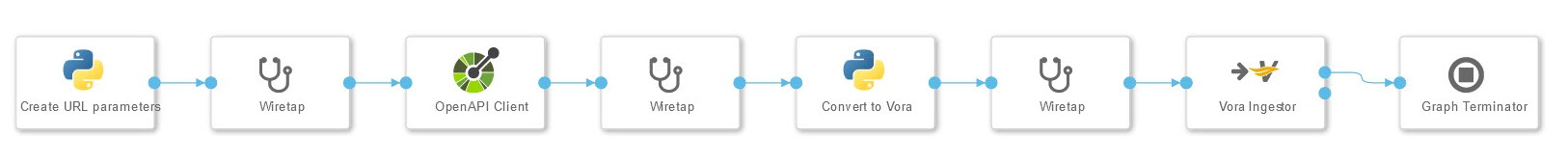
Im ersten Transformationsszenario wurden Daten von einer Website geladen und in einem VORA File abgelegt. Für die Verbindung zur Website wird der Open API Client genutzt. Die Query, die an diesen gesendet wird, sowie die anschließende Transformation werden mit einem Python Operator erstellt, der jeweils eigenes Coding beinhaltet. Die Transformation macht die Daten Vora-kompatibel. Wiretap-Operatoren, die zwischen die Operatoren geschaltet werden erlauben Debugging und die Zwischenergebnisse zu prüfen. Für die Produktivsetzung werden diese entfernt. Der Graph Terminator beendet den Graphen nach einmaligem Durchlauf.

ABAP Tabelle COEP via SLT mit Split in Kafka und HANA Tabelle

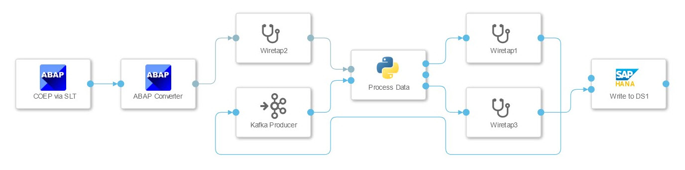
In diesem Szenario wurde die Verbindung zu einem SAP ECC System getestet, dessen Daten in die HANA geschrieben und mittels Kafka gestreamt werden sollen. Die Daten aus dem ECC Table wurden mittels SLT Connector gestreamt, der diese als JSON String an einen Python Operator übergibt. Dieser hat hier zwei Aufgaben. Er leitet die Daten an den HANA Client Operator und teilt die Daten in Pakete, die vom Kafka Producer verarbeitet werden können. Der Graph wird nicht per Operator beendet, sondern wartet auf weitere Daten. Das muss bei der Konfiguration der SLT Verbindung berücksichtigt werden, da die mehrfache Nutzung der gleichen Konfiguration zum Deadlock führen kann.

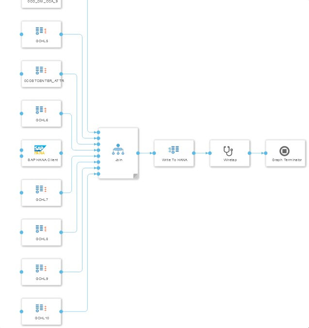
ECC Dataquelle gejoint mit hierarchischen Textdaten aus SQL-Server

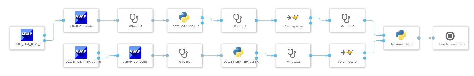
Im dritten Szenario wurden Bewegungsdaten aus einem ECC mit Stammdaten aus einem MS SQL-Server angereichert. Die Herausforderung für dieses Szenario ist es passende Einträge zu finden, ohne den gesamten Datensatz laden zu müssen. Für den Join wurden die Daten aus dem ECC ebenfalls in einer Datenbanktabelle gespeichert. Da die Information über die Verbindung zwischen Stamm- und Bewegungsdaten in einer weiteren ECC-Datenquelle lag wurde ein zweiter Graph erstellt. Der erste Graph zieht die Daten aus dem ECC, der zweite Graph erstellt den Join zwischen den beiden Tabellen aus dem ECC und den sechs Tabellen aus dem SQL-Server.

SAP BW Extraktion in zwei verschiedene HANA Datenbanken

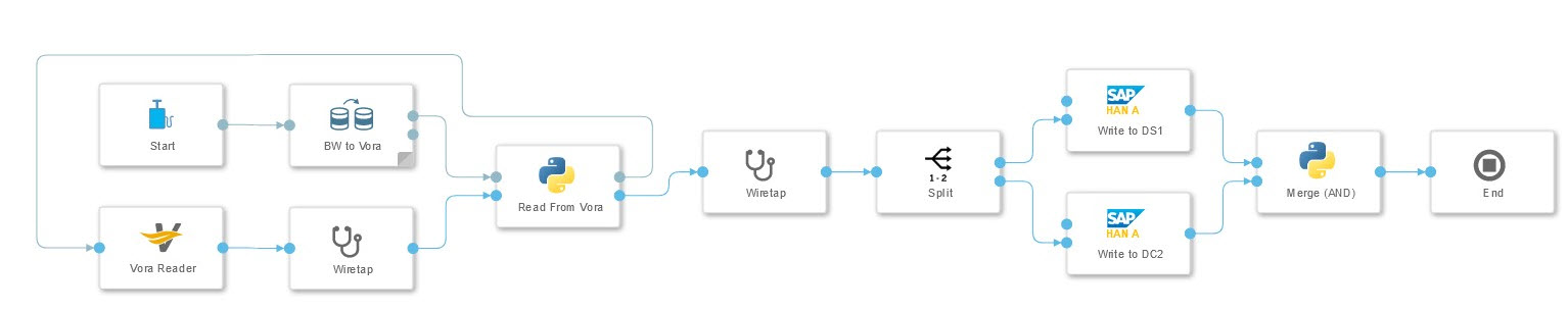
Die Extraktion von Daten aus dem SAP BW und das Schreiben in zwei unterschiedliche HANA Datenbanken wurde in diesem Szenario untersucht. Die Extraktion erfolgt mittels eines vorgefertigten Operators, der Daten in die Vora schreibt. Dessen Ergebnis kann von einem Python-Operator ausgelesen werden, der die Daten transformiert und an zwei separate HANA Clients übergibt. Der letzte Python Operator wartet auf die Erfolgsmeldungen beider HANA Clients bevor er durch eine Nachricht an den Terminator-Operator den Graphen beendet.

Kafka Nachrichten lesen, transformieren und in S3 Dateien schreiben

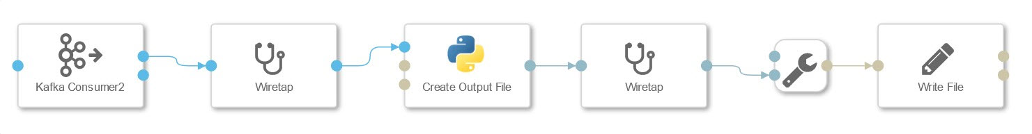
Hier wurde das Lesen von Datenpaketen aus Kafka und die Speicherung als S3 Datei getestet. Die ankommenden Pakete werden mittels Python-Operator in das csv-Format transformiert. Das erlaubt angebundene Spark oder Vora Systeme performant anzuschließen. Zu Testzwecken wurden Informationen aus dem Header wie Zeitstempel und Reihenfolge der Datenpakete mit herausgelesen. Der Header der ausgegebenen Datei kann ebenfalls angepasst werden um Informationen wie bspw. Spaltennamen mitzugeben.

Fazit

Auch wenn einige Aspekte noch nicht völlig ausgereift sind zum Zeitpunkt der Projektdurchführung, kann SAP DI für die Daten-Orchestrierung im Unternehmen empfohlen werden. Flexibilität spielt hierbei eine zentrale Rolle. Flexibilität entsteht durch eine große Zahl vorgefertigter Operatoren, die viele verschiedene Anwendungsszenarien bereits abdecken, als auch durch die Möglichkeit eigene Operatoren mit Customcode zu erstellen. Flexibilität entsteht auch durch die Basierung des Systems auf Containern, welche Skalierung und Parallelisierung erlauben.

Insbesondere die gute Integration mit bestehenden SAP-Lösungen hebt das Tool deutlich von anderen Anbietern ab, ohne die Integration von 3rd Party Lösungen zu vernachlässigen. Dies gepaart mit einer konsequenten Cloud-Nutzung und -Integration zeigt, dass das Tool ein Schritt in die richtige Richtung ist.

Ansprechpartner

Oliver Ossenbrink

Geschäftsführung Vertrieb und HR

Data Products Setup

I’ll start with Data Products setup. If you’re new to the concept, this recent video is a great starting point, but here’s a short summary. A data product is a well-described, easily discoverable, and consumable collection of data sets.

Creating a Data Product in Datasphere

Note that in this article I create Data Products in the Data Sharing Cockpit in Datasphere. This functionality is expected to move into the Data Product Studio, but that had not taken place at the time writing.

Before creating a Data Product in Datasphere, I need to set up a Data Provider profile, collecting descriptive metadata like contact and address details, industry, regional coverage, and importantly define Data Product Visibility. Enabling Formations allows me to share the Data Product with systems across your BDC Formation – Databricks, in this case.

With the Data Provider set up, I can go ahead and create a Data Product. As with the Data Provider, I’ll need to add metadata about the product and define its artifacts – the datasets it contains. Only datasets from a space of SAP HANA Data Lake Files type can be selected. Since this Data Product is visible across the Formation, it is available free of charge.

For this demo, the artifact is a local table containing ten years of Ice Cream sales data. Since this is a File type space, importing a CSV file directly to create a local table isn’t an option (see documentation).

I used a Replication Flow to perform an initial load from a BW aDSO table into a local table.

Once Data Product is created and listed, it becomes available in the Catalog & Marketplace, from where it can be shared with Databricks by selecting the appropriate connection details.

Jump into Databricks

To use the shared object In Databricks, I need to mount it to the Catalog – either by creating a new Catalog or using an existing one.

Databricks appends a version number to the end of the schema – ‘:v1’ – to maintain versioning in case of any future changes to the Data Product.

Once the share is mounted, the schema is created automatically, and the Sales actual data table becomes available within it. From there, I can access the shared table directly in a Notebook.

Creating a Data Product in Databricks

To create a Data Product in Databricks, I first need to create a Share – which I can either do via the Delta Sharing settings in the Catalog:

Or directly out of the table which is going to become a part of the Share:

Since a single Share can contain multiple tables, I have the option to either add the table to an existing Share, or create a new one:

To publish the Share as a Data Product, I run a Python script where I define the target table for the forecast and describe the Share in CSN notation, setting the Primary Keys. Primary Keys are required for installing Data Products in Datasphere.

Jump back into Datasphere

Once the Databricks Data Product is available in Datasphere, I install it into a Space configured as a HANA Database space – since my intention is to build a view on top of the table and use it for planning in SAC.

There are two installation options: as a Remote table for live data access, or as a Replication Flow, in which case the data is physically copied into the object store in Datasphere.

Since I want live access, I install it as a Remote Table:

and build a Graphical view of type Fact on top:

Forecast calculation

With my Data Products set up and Sales actual data are available in Databricks, I create a Notebook to calculate the Sales Forecast.

The approach combines Sales and Weather data to train a Linear Regression model. I import the Weather data *https://zenodo.org/records/4770937 from an external server directly into Databricks, select the relevant features from the weather dataset, and combine them with the Sales actual data:

* Klein Tank, A.M.G. and Coauthors, 2002. Daily dataset of 20th-century surface
air temperature and precipitation series for the European Climate Assessment.
Int. J. of Climatol., 22, 1441-1453.
Data and metadata available at http://www.ecad.eu

Using the “sklearn” library, I build and train a Linear regression model:

Once trained, the model predicts the Sales forecast for Rome in June 2026 based on the weather forecast, and I save the results to my Catalog table:

Seamless planning data model

Seamless planning concept is built around physically storing planning data and public dimensions directly in Datasphere, keeping them alongside the actual data.

Since the QRC4 2025 SAC release, it has also been possible to use live versions and bring reference data into planning models without replication.

In this scenario, I build a seamless planning model on top of the Graphical view I created over the Remote table. This lets me use the forecast generated in Databricks as a reference for the final SAC Forecast version.

The model setup follows these steps:

Create a new model:

Start with data:

Select Datasphere as the data storage:

From there, I define the model structure and can review the data in the preview.

For a deeper dive into Seamless Planning, I recommend this biX blog.

Process Flow automation

Multi-action triggers Datasphere task chain

The final step is automating the entire forecast generation by using SAC Multi-actions and a Task-Chain in Datasphere – so that my user can trigger the calculation with a single button click from an SAC Story.

The model setup follows these steps:

Create a new model:

Triggering Task Chains from Multi-actions is a recent release. This blog post walks through how to set it up.

For details on how to trigger a Databricks Notebook from Datasphere, I recommend referring to this blog.

With everything in place, I create a Story, add my Seamless planning Model, and attach the Multi-action:

Running the Multi-action triggers the Task Chain, which in turn triggers the Databricks Notebook.

I can monitor the execution details in Datasphere:

and in Databricks:

Once the calculation completes, the updated forecast appears in the Story:

The end-to-end calculation took 2 minutes 45 seconds in total. The Task Chain in Datasphere is triggered almost instantly by the Multi-action, the Databricks Notebook execution itself took 1 minute 29 seconds, with the remaining time spent on Serverless Cluster startup.

From here, I can copy the calculated forecast into a new private version:

adjust the numbers as needed, and publish it as a new public version to Datasphere:

Conclusion

With SAP Business Data Cloud, it is possible to build a forecasting workflow that feels seamless to the end user — even though it spans multiple systems under the hood.

Companies using BW as the main Data Warehouse and Databricks for ML calculations or Data Science tasks can benefit from using the platform, as the data no longer needs to be physically copied out of BW.

What this scenario demonstrates is that once wrapped as a Data Product, BW sales data can be shared with Databricks via the Delta Share protocol. Databricks, in turn, can then create its own Data Products on top of the calculation results and share them back with Datasphere as a Remote Table.

A Seamless Planning model in SAC sits on top of that Remote Table, giving planners live access to the generated forecast. A single Multi-action in an SAC Story ties it all together, triggering a Datasphere Task Chain that kicks off the Databricks Notebook — completing the full cycle in under three minutes.

As SAP Business Data Cloud continues to mature, scenarios like this one are becoming achievable – leaving the complexity in the architecture and not in the workflow.