biX AI Tools – Fallbeispiel: Customer-Churn-Prevention

Customer-Churn ist die vom Kunden ausgehende Kündigung. Die Vorhersage solcher Ereignisse vor dem Eintreten ist in vielen Geschäftsbereichen von großem Interesse. Die Fokussierung von Gegenmaßnahmen auf relevante Kunden verringert den Aufwand und verhindert einen Schläfereffekt bei nicht gefährdeten Kunden.

Ein möglicher Weg zur Vorhersage von Churn soll hier mittels Decision Trees aus der SAP HANA Predictive Analysis Library (PAL) gezeigt werden. Als Datengrundlage dient ein Datenset von Kundendaten eines Telekommunikations- unternehmens mit bekannten Churn-Ereignissen.

Der Schläfereffekt beschreibt, dass Kunden erst durch den hergestellten Kontakt ihre Vertragsbedingungen bewerten und daraufhin kündigen.

Ein Decision Tree trennt den Datensatz möglichst genau in Churn-Kunden und Nicht-Churn-Kunden. Dafür erstellt er Entscheidungsregeln, für die er Kundenmerkmale verwendet, wie z.B. „Monatlicher Umsatz > X“ oder „Nutzung von Streamingangeboten Ja/Nein“. Die Kombination der Einzelregeln erlaubt dem Decision Tree dann schließlich die Zuordnung eines Kunden zu Churn/ Nicht-Churn.

Abbildung 1: Ausschnitt aus möglichem Decision Tree

Die Auswahl der Parameter bei der Erstellung eines Decision Trees beeinflusst sowohl die Genauigkeit der Zuordnung als auch die Komplexität der Regeln. Setzt man den Wert der Einfachheit hoch, so werden die Regeln weniger spezifisch, aber die Genauigkeit der Klassifizierung nimmt meist ab. Es gilt also zwischen Lesbarkeit und besserer Trennung abzuwägen.

Einfachheit beschreibt hier die nötige Zahl der Kunden, die mit einer Regel beschrieben werden. Wird dieser Wert nicht erreicht, so wird die Regel nicht gebildet und die weitere Aufteilung endet in diesem Zweig.

Für die Erstellung des Decision Trees und die Überprüfung der erstellten Regeln werden Trainings- und Testdatensets benötigt. In diesem Beispiel liegt der Datensatz in einem aDSO im SAP BW vor. Trainingsset und Testset werden für die Vergleichbarkeit von Durchläufen aus dem Datensatz als Tabellen persistiert. Die Datenvorverarbeitung und die Aufteilung der Daten erfolgten mittels ABAP.

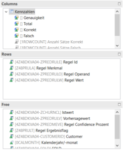
Nach der Erstellung der getrennten Sets wird die Qualität der erstellten Decision Trees zunächst mit dem Trainings- dann mit dem Testset beurteilt. Bei zufriedenstellender Genauigkeit der Trennung von Churn und Nicht-Churn wird ein finaler Decision Tree auf gemeinsamer Basis von Trainings- und Testdaten erstellt. Die Decision Trees werden mit einem Aufruf der SAP HANA PAL in ABAP erstellt. Die erstellten und kombinierten Regeln aus der PAL sind ohne weitere Formatierung nur schwer lesbar und noch nicht einzelnen Kunden zugeordnet. Für die Überprüfung der richtigen Anwendung der Stamm- und Bewegungsdaten in den Regeln ist ein Einblick aber wünschenswert. Zudem kann die Betrachtung, welche Regel für einen Kunden gilt, Hinweise darauf geben, welche Aspekte das Churn-Ereignis abwenden können. Daher werden die Regeln in weiteren ABAP-Programmen formatiert und jedem Kunden die angewendete Regel zugeordnet. Die aufbereiteten Regeln werden mit den Kundendaten in einem aDSO zusammengeführt und können per Query ausgewertet werden.

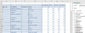
Mit einer Einfachheit von 150 wird eine Genauigkeit von über 75% über den gesamten Datensatz erreicht. Die Betrachtung auf Regelebene erlaubt aber auch die Bewertung der Genauigkeit der einzelnen Regeln, die auch mehr als 90% erreichen kann.

So können die Maßnahmen für die Churn-Prevention auf gefährdete Kunden mit ausreichender Vorhersagegenauigkeit fokussiert werden. Dadurch können Kosten für Vertriebsmaßnahmen verringert und die Effizienz durch die Vermeidung falscher Kundenkontakte erhöht werden.

Ansprechpartner

Oliver Ossenbrink

Geschäftsführung Vertrieb und HR

Data Products Setup

I’ll start with Data Products setup. If you’re new to the concept, this recent video is a great starting point, but here’s a short summary. A data product is a well-described, easily discoverable, and consumable collection of data sets.

Creating a Data Product in Datasphere

Note that in this article I create Data Products in the Data Sharing Cockpit in Datasphere. This functionality is expected to move into the Data Product Studio, but that had not taken place at the time writing.

Before creating a Data Product in Datasphere, I need to set up a Data Provider profile, collecting descriptive metadata like contact and address details, industry, regional coverage, and importantly define Data Product Visibility. Enabling Formations allows me to share the Data Product with systems across your BDC Formation – Databricks, in this case.

With the Data Provider set up, I can go ahead and create a Data Product. As with the Data Provider, I’ll need to add metadata about the product and define its artifacts – the datasets it contains. Only datasets from a space of SAP HANA Data Lake Files type can be selected. Since this Data Product is visible across the Formation, it is available free of charge.

For this demo, the artifact is a local table containing ten years of Ice Cream sales data. Since this is a File type space, importing a CSV file directly to create a local table isn’t an option (see documentation).

I used a Replication Flow to perform an initial load from a BW aDSO table into a local table.

Once Data Product is created and listed, it becomes available in the Catalog & Marketplace, from where it can be shared with Databricks by selecting the appropriate connection details.

Jump into Databricks

To use the shared object In Databricks, I need to mount it to the Catalog – either by creating a new Catalog or using an existing one.

Databricks appends a version number to the end of the schema – ‘:v1’ – to maintain versioning in case of any future changes to the Data Product.

Once the share is mounted, the schema is created automatically, and the Sales actual data table becomes available within it. From there, I can access the shared table directly in a Notebook.

Creating a Data Product in Databricks

To create a Data Product in Databricks, I first need to create a Share – which I can either do via the Delta Sharing settings in the Catalog:

Or directly out of the table which is going to become a part of the Share:

Since a single Share can contain multiple tables, I have the option to either add the table to an existing Share, or create a new one:

To publish the Share as a Data Product, I run a Python script where I define the target table for the forecast and describe the Share in CSN notation, setting the Primary Keys. Primary Keys are required for installing Data Products in Datasphere.

Jump back into Datasphere

Once the Databricks Data Product is available in Datasphere, I install it into a Space configured as a HANA Database space – since my intention is to build a view on top of the table and use it for planning in SAC.

There are two installation options: as a Remote table for live data access, or as a Replication Flow, in which case the data is physically copied into the object store in Datasphere.

Since I want live access, I install it as a Remote Table:

and build a Graphical view of type Fact on top:

Forecast calculation

With my Data Products set up and Sales actual data are available in Databricks, I create a Notebook to calculate the Sales Forecast.

The approach combines Sales and Weather data to train a Linear Regression model. I import the Weather data *https://zenodo.org/records/4770937 from an external server directly into Databricks, select the relevant features from the weather dataset, and combine them with the Sales actual data:

* Klein Tank, A.M.G. and Coauthors, 2002. Daily dataset of 20th-century surface
air temperature and precipitation series for the European Climate Assessment.
Int. J. of Climatol., 22, 1441-1453.
Data and metadata available at http://www.ecad.eu

Using the “sklearn” library, I build and train a Linear regression model:

Once trained, the model predicts the Sales forecast for Rome in June 2026 based on the weather forecast, and I save the results to my Catalog table:

Seamless planning data model

Seamless planning concept is built around physically storing planning data and public dimensions directly in Datasphere, keeping them alongside the actual data.

Since the QRC4 2025 SAC release, it has also been possible to use live versions and bring reference data into planning models without replication.

In this scenario, I build a seamless planning model on top of the Graphical view I created over the Remote table. This lets me use the forecast generated in Databricks as a reference for the final SAC Forecast version.

The model setup follows these steps:

Create a new model:

Start with data:

Select Datasphere as the data storage:

From there, I define the model structure and can review the data in the preview.

For a deeper dive into Seamless Planning, I recommend this biX blog.

Process Flow automation

Multi-action triggers Datasphere task chain

The final step is automating the entire forecast generation by using SAC Multi-actions and a Task-Chain in Datasphere – so that my user can trigger the calculation with a single button click from an SAC Story.

The model setup follows these steps:

Create a new model:

Triggering Task Chains from Multi-actions is a recent release. This blog post walks through how to set it up.

For details on how to trigger a Databricks Notebook from Datasphere, I recommend referring to this blog.

With everything in place, I create a Story, add my Seamless planning Model, and attach the Multi-action:

Running the Multi-action triggers the Task Chain, which in turn triggers the Databricks Notebook.

I can monitor the execution details in Datasphere:

and in Databricks:

Once the calculation completes, the updated forecast appears in the Story:

The end-to-end calculation took 2 minutes 45 seconds in total. The Task Chain in Datasphere is triggered almost instantly by the Multi-action, the Databricks Notebook execution itself took 1 minute 29 seconds, with the remaining time spent on Serverless Cluster startup.

From here, I can copy the calculated forecast into a new private version:

adjust the numbers as needed, and publish it as a new public version to Datasphere:

Conclusion

With SAP Business Data Cloud, it is possible to build a forecasting workflow that feels seamless to the end user — even though it spans multiple systems under the hood.

Companies using BW as the main Data Warehouse and Databricks for ML calculations or Data Science tasks can benefit from using the platform, as the data no longer needs to be physically copied out of BW.

What this scenario demonstrates is that once wrapped as a Data Product, BW sales data can be shared with Databricks via the Delta Share protocol. Databricks, in turn, can then create its own Data Products on top of the calculation results and share them back with Datasphere as a Remote Table.

A Seamless Planning model in SAC sits on top of that Remote Table, giving planners live access to the generated forecast. A single Multi-action in an SAC Story ties it all together, triggering a Datasphere Task Chain that kicks off the Databricks Notebook — completing the full cycle in under three minutes.

As SAP Business Data Cloud continues to mature, scenarios like this one are becoming achievable – leaving the complexity in the architecture and not in the workflow.